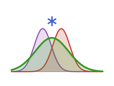
Visualising convolutions

Introduction

This tutorial shows what the package does by plotting it. A Convolved distribution is the sum of independent delays, so its density sits to the right of, and is wider than, either component. A Difference is the signed gap between two events, so its support runs on both sides of zero. The plots below make each of these behaviours visible, and also check the analytic and numeric solver backends against each other.

What are we going to do in this exercise

1. Overlay two component densities with their convolved density.

2. Plot the density of the difference of the same pair across zero.

3. Compare the analytic and numeric solver CDFs and plot their residual.

4. Compare a right-truncated convolution with the untruncated density.

5. Convolve a synthetic infection curve into an expected count curve.

What might I need to know before starting

This tutorial builds on the Getting started overview and uses AlgebraOfGraphics.jl and CairoMakie.jl for plotting. No fitting or MCMC is involved; every quantity is a direct evaluation.

Packages used

using ConvolvedDistributions, Distributions
using CairoMakie, AlgebraOfGraphics, DataFramesMeta

CairoMakie.activate!(type = "png", px_per_unit = 2)

Two components and their sum

We use a Gamma incubation period and a LogNormal reporting delay, a pair with no closed-form convolution, so the density comes from the quadrature path. convolved returns the distribution of the sum, and the batched pdf method evaluates a whole grid with a single quadrature solve.

incubation = Gamma(2.0, 1.0)
reporting = LogNormal(1.0, 0.5)
d = convolved(incubation, reporting)

x = 0.0:0.05:15.0
components_df = vcat(
    DataFrame(x = x, density = pdf.(incubation, x),
        Distribution = "Incubation (Gamma)"),
    DataFrame(x = x, density = pdf.(reporting, x),
        Distribution = "Reporting (LogNormal)"),
    DataFrame(x = x, density = pdf(d, collect(x)),
        Distribution = "Convolved sum")
)
draw(
    data(components_df) *
    mapping(:x, :density, color = :Distribution) *
    visual(Lines, linewidth = 2);
    axis = (xlabel = "Delay (days)", ylabel = "Density")
)

The convolved density peaks later than either component and is flatter, because summing independent delays adds both their means and their variances.

The difference of the same pair

difference builds Z = X - Y, here the reporting delay minus the incubation period. Reflecting the subtracted component makes the support two-sided, so the density crosses zero.

z_dist = difference(reporting, incubation)
z = -8.0:0.05:12.0
difference_df = DataFrame(z = z, density = pdf.(z_dist, z))
draw(
    data(difference_df) *
    mapping(:z, :density) *
    visual(Lines, linewidth = 2);
    axis = (xlabel = "Reporting delay - incubation period (days)",
        ylabel = "Density")
)

The mass below zero is the probability that the reporting delay is shorter than the incubation period.

cdf(z_dist, 0.0)

0.2801512628537788

Analytic and numeric solvers agree

For an equal-scale Gamma pair a closed-form convolution exists and the default AnalyticalSolver uses it. Passing NumericSolver forces the quadrature path on the same pair, which lets us check the numeric machinery against the exact answer.

pair = (Gamma(2.0, 1.0), Gamma(3.0, 1.0))
d_analytic = convolved(pair...)
d_numeric = convolved(pair...; method = NumericSolver())

xs = 0.0:0.1:20.0
solver_df = vcat(
    DataFrame(x = xs, cdf = cdf(d_analytic, collect(xs)),
        Solver = "Analytic (closed form)"),
    DataFrame(x = xs, cdf = cdf(d_numeric, collect(xs)),
        Solver = "Numeric (quadrature)")
)
draw(
    data(solver_df) *
    mapping(:x, :cdf, color = :Solver, linestyle = :Solver) *
    visual(Lines, linewidth = 2);
    axis = (xlabel = "Delay (days)", ylabel = "CDF")
)

The two curves lie on top of each other, so we plot the residual to see the actual size of the quadrature error.

residual_df = DataFrame(x = xs,
    residual = cdf(d_numeric, collect(xs)) .- cdf(d_analytic, collect(xs)))
draw(
    data(residual_df) *
    mapping(:x, :residual) *
    visual(Lines, linewidth = 2);
    axis = (xlabel = "Delay (days)",
        ylabel = "Numeric CDF - analytic CDF")
)

The largest absolute residual across the grid is a few parts in a million, the size of the fixed-node quadrature error and its tail clamp.

maximum(abs, residual_df.residual)

2.7099473987324263e-6

Truncation composes

A Convolved distribution is a UnivariateDistribution, so Distributions.truncated applies directly. Right truncation renormalises the density over the kept region, which is the correction needed when scoring against data observed only up to a cutoff.

d_trunc = truncated(d; upper = 10.0)
truncation_df = vcat(
    DataFrame(x = x, density = pdf(d, collect(x)),
        Distribution = "Convolved"),
    DataFrame(x = x, density = pdf.(d_trunc, x),
        Distribution = "Truncated at 10")
)
draw(
    data(truncation_df) *
    mapping(:x, :density, color = :Distribution) *
    visual(Lines, linewidth = 2);
    axis = (xlabel = "Delay (days)", ylabel = "Density")
)

The truncated density is zero beyond the cutoff and sits above the untruncated density below it, since the removed tail mass is redistributed over the kept region.

Timeseries convolution

The timeseries form convolve_series(delay, series) discretises the delay to a PMF on the unit grid and convolves a numeric series with it. With the series an expected infection curve, the result is the expected downstream count curve, the renewal-style observation layer.

t = 0:40
infections = 100 .* exp.(-((t .- 12.0) .^ 2) ./ 30.0)
expected = convolve_series(d, infections)

timeseries_df = vcat(
    DataFrame(t = t, count = infections, Series = "Infections"),
    DataFrame(t = t, count = expected, Series = "Expected reports")
)
draw(
    data(timeseries_df) *
    mapping(:t, :count, color = :Series) *
    visual(Lines, linewidth = 2);
    axis = (xlabel = "Day", ylabel = "Expected count")
)

The report curve is shifted right by the mean total delay and is flatter than the infection curve, because convolution smears each day's infections across the delay distribution. Mass delayed beyond the series window is truncated rather than renormalised, so the report curve carries slightly less total mass.

Summary

• Convolving two delays shifts and widens the density; the batched pdf and cdf methods evaluate a grid in one quadrature solve.

• difference has two-sided support and its mass below zero is directly interpretable as an ordering probability.

• Forcing the NumericSolver on an analytic pair reproduces the closed-form CDF to a few parts in a million.

• truncated composes with a Convolved distribution for scoring under right truncation.

• The timeseries form turns an infection curve into an expected count curve through the discretised delay PMF.