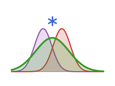
Convolving distributions

Introduction

This tutorial shows what convolved does by plotting it. A Convolved distribution is the sum of independent delays, so its density sits to the right of, and is wider than, either component. The plots below make that visible, check that a nested convolution matches its flat equivalent, and check the analytic and numeric solver backends against each other.

What are we going to do in this exercise

2. Overlay two component densities with their convolved density.

3. Nest one convolution inside another and check it against the flat form.

4. Compare the analytic and numeric solver CDFs and plot their residual.

5. Compare a right-truncated convolution with the untruncated density.

What might I need to know before starting

This tutorial builds on the Getting started overview and uses AlgebraOfGraphics.jl and CairoMakie.jl for plotting. No fitting or MCMC is involved; every quantity is a direct evaluation.

Packages used

using ConvolvedDistributions, Distributions
using CairoMakie, AlgebraOfGraphics, DataFramesMeta

CairoMakie.activate!(type = "png", px_per_unit = 2)

Two components and their sum

We use a Gamma incubation period and a LogNormal reporting delay, a pair with no closed-form convolution, so the density comes from the quadrature path. convolved returns the distribution of the sum, and the batched pdf method evaluates a whole grid with a single quadrature solve.

incubation = Gamma(2.0, 1.0)
reporting = LogNormal(1.0, 0.5)
d = convolved(incubation, reporting)

x = 0.0:0.05:15.0
components_df = vcat(
    DataFrame(
        x = x, density = pdf.(incubation, x),
        Distribution = "Incubation (Gamma)"
    ),
    DataFrame(
        x = x, density = pdf.(reporting, x),
        Distribution = "Reporting (LogNormal)"
    ),
    DataFrame(
        x = x, density = pdf(d, collect(x)),
        Distribution = "Convolved sum"
    )
)
draw(
    data(components_df) *
        mapping(:x, :density, color = :Distribution) *
        visual(Lines, linewidth = 2);
    axis = (xlabel = "Delay (days)", ylabel = "Density")
)

The convolved density peaks later than either component and is flatter, because summing independent delays adds both their means and their variances.

Composing on multiple distributions

A Convolved distribution is itself a UnivariateDistribution, so it can be a component of another convolved call. Here the two-stage delay d gains an Exponential processing stage, built once by nesting (convolved(d, processing)) and once flat from the three leaves.

processing = Exponential(2.0)
total_nested = convolved(d, processing)
total_flat = convolved(incubation, reporting, processing)

xn = 0.0:0.25:20.0
nested_df = vcat(
    DataFrame(
        x = xn, density = pdf(d, collect(xn)),
        Distribution = "Two-stage delay"
    ),
    DataFrame(
        x = xn, density = pdf(total_nested, collect(xn)),
        Distribution = "Nested three-stage"
    ),
    DataFrame(
        x = xn, density = pdf(total_flat, collect(xn)),
        Distribution = "Flat three-stage"
    )
)
draw(
    data(nested_df) *
        mapping(
        :x, :density,
        color = :Distribution, linestyle = :Distribution
    ) *
        visual(Lines, linewidth = 2);
    axis = (xlabel = "Delay (days)", ylabel = "Density")
)

The nested and flat densities coincide, and adding the third stage shifts and widens the two-stage density. The quadrature folds the flat component tuple recursively, so the two forms evaluate the same integral; the moments are exact component sums either way.

mean(total_nested), mean(total_flat)

(7.080216848918031, 7.080216848918031)

Analytic and numeric solvers agree

For an equal-scale Gamma pair a closed-form convolution exists and the default AnalyticalSolver uses it. Passing NumericSolver forces the quadrature path on the same pair, which lets us check the numeric machinery against the exact answer.

pair = (Gamma(2.0, 1.0), Gamma(3.0, 1.0))
d_analytic = convolved(pair...)
d_numeric = convolved(pair...; method = NumericSolver())

xs = 0.0:0.1:20.0
solver_df = vcat(
    DataFrame(
        x = xs, cdf = cdf(d_analytic, collect(xs)),
        Solver = "Analytic (closed form)"
    ),
    DataFrame(
        x = xs, cdf = cdf(d_numeric, collect(xs)),
        Solver = "Numeric (quadrature)"
    )
)
draw(
    data(solver_df) *
        mapping(:x, :cdf, color = :Solver, linestyle = :Solver) *
        visual(Lines, linewidth = 2);
    axis = (xlabel = "Delay (days)", ylabel = "CDF")
)

The two curves lie on top of each other, so we plot the residual to see the actual size of the quadrature error.

residual_df = DataFrame(
    x = xs,
    residual = cdf(d_numeric, collect(xs)) .- cdf(d_analytic, collect(xs))
)
draw(
    data(residual_df) *
        mapping(:x, :residual) *
        visual(Lines, linewidth = 2);
    axis = (
        xlabel = "Delay (days)",
        ylabel = "Numeric CDF - analytic CDF",
    )
)

The largest absolute residual across the grid is a few parts in a million, the size of the fixed-node quadrature error and its tail clamp.

maximum(abs, residual_df.residual)

7.771561172376096e-16

Custom solver payloads

Beyond the binary AnalyticalSolver/NumericSolver choice, a solver can carry a custom payload that the numeric path honours. NumericSolver (or AnalyticalSolver) takes an optional quadrature solver; a non-default GaussLegendre raises the nodal accuracy. With the optional Integrals.jl extension loaded, an Integrals.jl algorithm such as NumericSolver(Integrals.QuadGKJL()) routes the integration window through IntegralProblem/solve.

using ConvolvedDistributions: GaussLegendre
using Integrals: QuadGKJL

A higher-node GaussLegendre payload raises accuracy; here a 256-node rule agrees with the default to machine precision.

pair = (Gamma(2.0, 1.0), LogNormal(0.5, 0.4))
d_default = convolved(pair...)
d_custom = convolved(pair...; method = NumericSolver(GaussLegendre(; n = 256)))
d_quadgk = convolved(pair...; method = NumericSolver(QuadGKJL()))

cdf_default = cdf(d_default, 5.0)
cdf_custom = cdf(d_custom, 5.0)
cdf_quadgk = cdf(d_quadgk, 5.0)
(cdf_default, cdf_custom, cdf_quadgk, cdf_quadgk - cdf_default)

(0.8051810060082844, 0.805181006008284, 0.8051810060082842, -1.1102230246251565e-16)

Truncation composes

A Convolved distribution is a UnivariateDistribution, so Distributions.truncated applies directly. Right truncation renormalises the density over the kept region, which is the correction needed when scoring against data observed only up to a cutoff.

d_trunc = truncated(d; upper = 10.0)
truncation_df = vcat(
    DataFrame(
        x = x, density = pdf(d, collect(x)),
        Distribution = "Convolved"
    ),
    DataFrame(
        x = x, density = pdf.(d_trunc, x),
        Distribution = "Truncated at 10"
    )
)
draw(
    data(truncation_df) *
        mapping(:x, :density, color = :Distribution) *
        visual(Lines, linewidth = 2);
    axis = (xlabel = "Delay (days)", ylabel = "Density")
)

The truncated density is zero beyond the cutoff and sits above the untruncated density below it, since the removed tail mass is redistributed over the kept region.

Summary

• Convolving two delays shifts and widens the density; the batched pdf and cdf methods evaluate a grid in one quadrature solve.

• A Convolved can be a component of another convolution, and a nested convolution matches its flat equivalent.

• Forcing the NumericSolver on an analytic pair reproduces the closed-form CDF to a few parts in a million.

• truncated composes with a Convolved distribution for scoring under right truncation.

See also: The difference of two delays, The product of two delays, Convolving a timeseries.