ConvolvedDistributions

Raw-distribution convolution and shared numeric quadrature for any Distributions.jl distribution.

Why ConvolvedDistributions?

• A convolution is usually only available in closed form for a few matching distribution families; convolved builds the distribution of a sum of independent delays from any two or more Distributions.jl distributions, not just those pairs.

• Closed-form convolutions (Normal + Normal, equal-scale Gamma, equal-rate Exponential) are used where they exist, with an AD-safe Gauss-Legendre quadrature fallback for every other pair.

• Sums are not the only combination we support: difference builds the X - Y signed gap between two independent events, product the X * Y Mellin convolution for a delay scaled by an independent multiplicative factor, and ratio the X / Y quotient for a rate, a proportion, or a normalised measurement.

• Turning expected events into expected downstream counts is usually a hand-rolled discrete convolution; convolve_series does it directly from a numeric series and a delay's PMF, including a delay that changes over the series (one distribution or PMF per time point).

Getting started

See the Getting started documentation for a full walkthrough.

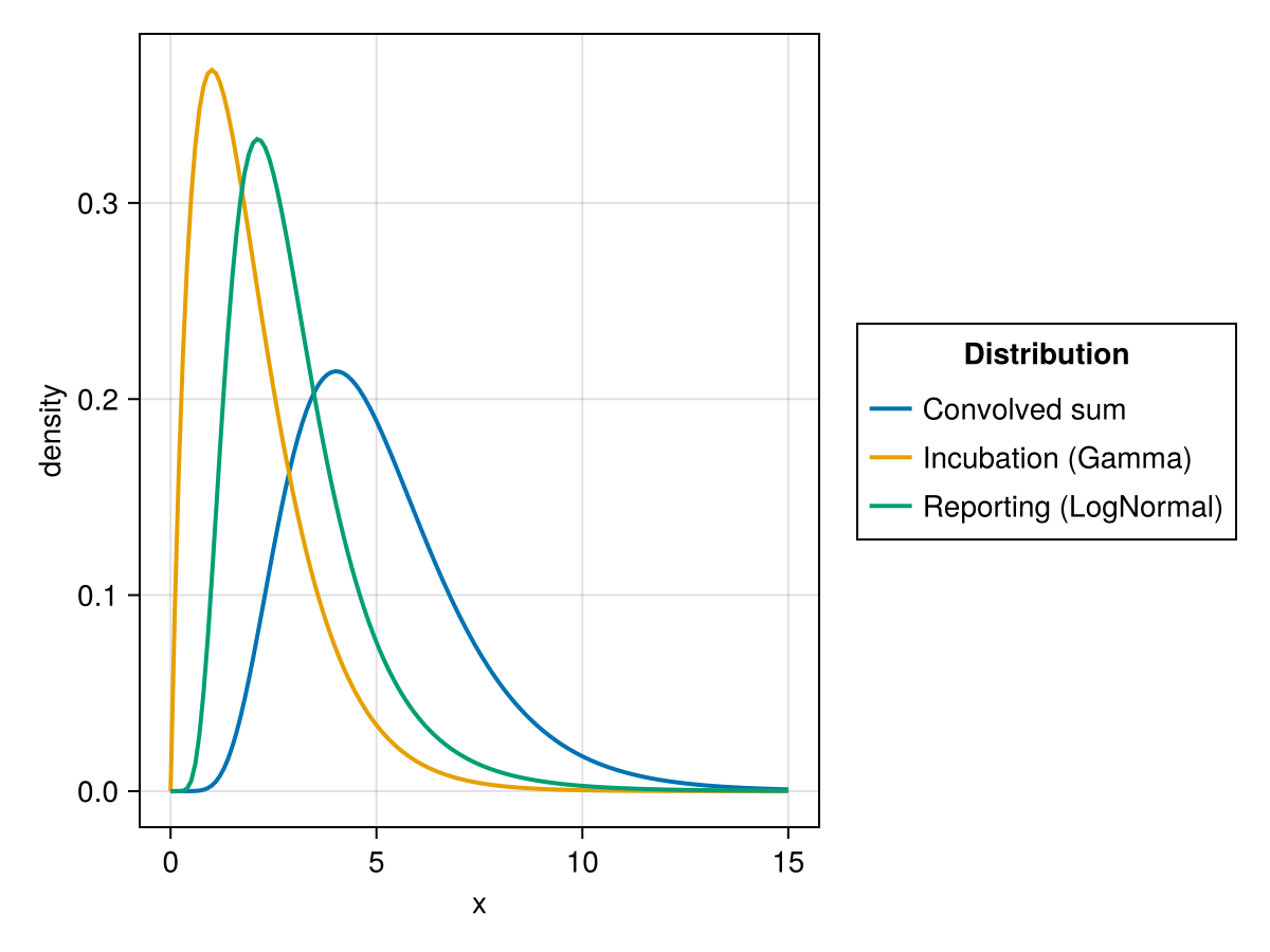
The following example convolves two delays, an incubation period and a reporting delay, and evaluates the resulting distribution:

using ConvolvedDistributions, Distributions

incubation = Gamma(2.0, 1.0)
reporting = LogNormal(1.0, 0.5)
d = convolved(incubation, reporting)

(cdf(d, 5.0), pdf(d, 5.0))

(0.5555707883725697, 0.18877150759921843)

difference gives the gap between two independent events:

z = difference(Normal(5.0, 1.0), Normal(2.0, 1.0))

(mean(z), cdf(z, 0.0))

(3.0, 0.016947426762344637)

A Convolved distribution is a UnivariateDistribution, so it composes with Distributions.truncated.

d_trunc = truncated(d; upper = 10.0)

cdf(d_trunc, 5.0)

0.5725523804006694

Loading the Optimization extension adds quantile support by numerically inverting the CDF:

using Optimization, OptimizationOptimJL

quantile(d, 0.5)

4.714710420969208

The components and their sum can be compared visually,

using CairoMakie, AlgebraOfGraphics, DataFramesMeta

CairoMakie.activate!(type = "png", px_per_unit = 2)

x = 0.0:0.1:15.0
df = vcat(
    DataFrame(x = x, density = pdf.(incubation, x),
        Distribution = "Incubation (Gamma)"),
    DataFrame(x = x, density = pdf.(reporting, x),
        Distribution = "Reporting (LogNormal)"),
    DataFrame(x = x, density = pdf(d, collect(x)),
        Distribution = "Convolved sum")
)
draw(
    data(df) *
    mapping(:x, :density, color = :Distribution) *
    visual(Lines, linewidth = 2)
)

Relationship to Distributions.jl

Distributions.jl ships a convolve function, but it only covers pairs with a closed-form result:

Aspect	Distributions.jl convolve	ConvolvedDistributions.jl convolved
Coverage	Closed-form, same-family pairs only (e.g. Normal + Normal, equal-scale Gamma); errors otherwise	Any pair of univariate distributions
Method	Returns the closed-form distribution	Analytic fast path where a closed form exists, AD-safe Gauss-Legendre quadrature fallback otherwise
Forms	Two positional arguments	Nested, vector, tuple, and varargs forms for sums of many delays
Differences	Not supported	difference builds the X - Y dual
Products	Not supported	product builds the X * Y Mellin convolution
Ratios	Not supported	ratio builds the X / Y Mellin-quotient form

For example, Distributions.convolve(Gamma(2, 1), LogNormal(0, 1)) throws a MethodError and Distributions.convolve(Gamma(2, 1), Gamma(3, 2)) throws an ArgumentError because the scales differ, whereas convolved handles both via quadrature. When a closed form does exist, convolved uses it.

Related packages

• ComposedDistributions.jl re-exports this package directly, so a composed chain collapses to its convolved total via observed_distribution.

• ModifiedDistributions.jl applies its forward-series transforms (thin, cumulative) to a convolved series, and lets modified distributions serve as convolution components.

• LoweredDistributions.jl lowers a convolved sum to one combined dynamical-systems representation, folding the components' phase-types in series rather than lowering each separately.

• CensoredDistributions.jl adds censoring and truncation layers for epidemiological observation processes; this package was split out of it, and convolve_series reads its double-interval-censored masses directly.

• DistributionsInference.jl is the emerging fit-protocol and PPL-integration layer across the EpiAware distribution packages.

Where to learn more

• Want to get started running code? Check out the Getting started documentation.

• Want to understand the API? Check out our API reference.

• Want to contribute to ConvolvedDistributions? Check the open issues and the Contributing section below.

• Want to see our code? Check out our GitHub Repository.

Getting help

For usage questions, ask on the Julia Discourse or the epinowcast community forum, our home for epidemiological modelling questions. Please use GitHub issues for bug reports and feature requests only.

Contributing

We welcome contributions and new contributors! This package follows ColPrac and is formatted with Runic.

Supporting and citing

If you would like to support ConvolvedDistributions, please star the repository — such metrics help secure future funding.

If you use ConvolvedDistributions in your work, please cite it:

@software{ConvolvedDistributions_jl,
  author       = {Sam Abbott and EpiAware contributors},
  title        = {ConvolvedDistributions.jl},
  year         = {2026},
  url          = {https://github.com/EpiAware/ConvolvedDistributions.jl}
}

A citable DOI will be added with the first tagged release.

Code of conduct

Please note that the ConvolvedDistributions project is released with a Contributor Code of Conduct. By contributing, you agree to abide by its terms.