The product of two delays
Introduction
A Product is the multiplicative member of the family: it builds Z = X * Y for independent X and Y, as when a delay is stretched by an independent multiplicative factor. Where Convolved (see Convolving distributions) sums two delays and Difference (see The difference of two delays) takes their signed gap, a product scales one variable by another.
What are we going to do in this exercise
Overlay two component densities with their product density.
Scale a Convolved two-stage delay by an independent factor.
Compare the analytic and numeric solver CDFs for a pair with a closed-form product and plot their residual.
What might I need to know before starting
This tutorial builds on the Getting started overview and uses AlgebraOfGraphics.jl and CairoMakie.jl for plotting. No fitting or MCMC is involved; every quantity is a direct evaluation.
Packages used
using ConvolvedDistributions, Distributions
using CairoMakie, AlgebraOfGraphics, DataFramesMeta

CairoMakie.activate!(type = "png", px_per_unit = 2)
Two components and their product
product returns the distribution of Z = X * Y, so both components must have non-negative support. The multiplier here is a dimensionless multiplicative factor rather than a delay, so the shared x-axis below is labelled "Value" rather than "Delay (days)": it is only a delay for the incubation and product curves.
incubation = Gamma(2.0, 1.0)
factor = LogNormal(0.0, 0.3)
w = product(incubation, factor)

x = 0.0:0.05:15.0
components_df = vcat(
    DataFrame(
        x = x, density = pdf.(incubation, x),
        Distribution = "Incubation (Gamma)"
    ),
    DataFrame(
        x = x, density = pdf.(factor, x),
        Distribution = "Multiplicative factor (LogNormal)"
    ),
    DataFrame(
        x = x, density = pdf(w, collect(x)),
        Distribution = "Product"
    )
)
draw(
    data(components_df) *
        mapping(:x, :density, color = :Distribution) *
        visual(Lines, linewidth = 2);
    axis = (xlabel = "Value", ylabel = "Density")
)
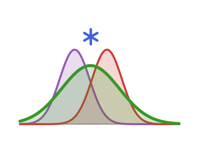
The product mean is the product of the component means, and the product density is wider and heavier-tailed than either component: multiplying by an independent factor stretches the spread as well as the centre.
mean(w), mean(incubation) * mean(factor)(2.092055719817434, 2.092055719817434)Scaling a Convolved delay
A Convolved distribution is itself a UnivariateDistribution, so it can be one side of a product. Here the two-stage delay incubation + reporting is scaled by an independent multiplicative factor.
reporting = LogNormal(1.0, 0.5)
d = convolved(incubation, reporting)
scaled = product(d, LogNormal(0.1, 0.25))

xn = 0.0:0.25:25.0
scaling_df = vcat(
    DataFrame(
        x = xn, density = pdf(d, collect(xn)),
        Distribution = "Two-stage delay"
    ),
    DataFrame(
        x = xn, density = pdf(scaled, collect(xn)),
        Distribution = "Scaled by factor"
    )
)
draw(
    data(scaling_df) *
        mapping(:x, :density, color = :Distribution) *
        visual(Lines, linewidth = 2);
    axis = (xlabel = "Delay (days)", ylabel = "Density")
)
The scaled mean is the two-stage delay's own mean multiplied by the factor's mean, and the scaled density is wider than the unscaled one, since scaling by an independent factor adds variance beyond what the factor's mean alone would suggest.
mean(d), mean(scaled)(5.080216848918031, 5.792731531720032)Analytic and numeric solvers agree
A LogNormal-LogNormal pair has a closed-form product (the log-parameters add) and the default AnalyticalSolver uses it. Passing NumericSolver forces the quadrature path on the same pair, which lets us check the numeric machinery against the exact answer.
pair = (LogNormal(0.0, 0.3), LogNormal(0.2, 0.4))
d_analytic = product(pair...)
d_numeric = product(pair...; method = NumericSolver())

xs = 0.05:0.05:8.0
solver_df = vcat(
    DataFrame(
        x = xs, cdf = cdf(d_analytic, collect(xs)),
        Solver = "Analytic (closed form)"
    ),
    DataFrame(
        x = xs, cdf = cdf(d_numeric, collect(xs)),
        Solver = "Numeric (quadrature)"
    )
)
draw(
    data(solver_df) *
        mapping(:x, :cdf, color = :Solver, linestyle = :Solver) *
        visual(Lines, linewidth = 2);
    axis = (xlabel = "Value", ylabel = "CDF")
)
The two curves lie on top of each other, so we plot the residual to see the actual size of the quadrature error.
residual_df = DataFrame(
    x = xs,
    residual = cdf(d_numeric, collect(xs)) .- cdf(d_analytic, collect(xs))
)
draw(
    data(residual_df) *
        mapping(:x, :residual) *
        visual(Lines, linewidth = 2);
    axis = (
        xlabel = "Value",
        ylabel = "Numeric CDF - analytic CDF",
    )
)
The largest absolute residual across the grid is a few parts in a billion, the size of the fixed-node quadrature error.
maximum(abs, residual_df.residual)7.89242227128284e-10Summary
Multiplying two delays scales both the mean and the spread of the resulting density; the batched
pdfandcdfmethods evaluate a grid in one quadrature solve.A
Convolvedcan be one side of aproduct, so a multi-stage delay scales by an independent factor in one call.Forcing the
NumericSolveron an analyticLogNormal-LogNormalpair reproduces the closed-form CDF to a few parts in a billion.
See also: Convolving distributions, The difference of two delays, Convolving a timeseries.